End-to-End Model-Based Autonomy for Building Energy Systems
Modern homes are getting a heat pump, a variable-speed compressor, time-of-use electricity prices, and — increasingly — a request from the grid to shed load at the wrong moment. A thermostat that simply chases a setpoint leaves comfort, energy, and money on the table. This project builds a full autonomy stack for residential HVAC that plans and controls the equipment the way a self-driving car plans and controls a vehicle: sense the world, forecast where it is going, generate a candidate action, and only actuate it after a safety check — with a proven fallback that always keeps the house under control.
The core idea is hybrid model-based control: physically-structured models (a grey-box thermal network for the room, physics-shaped capacity/power maps for the equipment) are learned from operating data, and the resulting optimal control problem is a hybrid program that mixes a continuous compressor speed with discrete on/off decisions. The whole stack is developed and validated against a high-fidelity EnergyPlus “virtual testbed” of a real house before it ever touches hardware.
1. Software architecture
The stack borrows the redundant-planner pattern from self-driving: a model-based optimizing planner, a rule-based fallback planner, and a selector/safety guardian that arbitrates between them. This gives optimization when it can be trusted and a field-proven fallback when it cannot — the system always degrades to a working controller, never to no control.
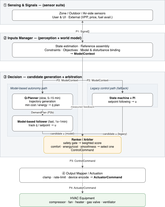
Four layers plus a measured-feedback loop, with a clean port contract between each stage:
| Layer | Role | Self-driving analogue |
|---|---|---|
| ① Sensing & Signals | raw per-device sources — zone/outdoor/air-side sensors, user & UI, external (VPP, price, fuel availability) | sensor suite |
| ② Inputs Manager | filter, validate, unit-normalize; state estimation; reference/constraint/objective assembly; bind models + disturbance forecasts → ModelContext |
perception + world model |
| ③ Decision | generate control candidates and arbitrate between them | prediction + planning + safety |
| ④ Output Mapper | clamp, rate-limit, dwell backstop, device encode → ActuatorCommand |
drive-by-wire |
The Decision layer is a three-part brain:
- Model-based path — the optimizing controller, itself two nested loops: a slow Q-Planner (5–15 min) that generates an economically-optimal heat-demand trajectory, and a fast follower (1 s–1 min) that tracks it on the equipment.
- Legacy path — a state-machine + PI controller that runs every tick, in parallel, producing a full candidate on the same schema. This is the minimal-risk guarantee: a fallback is always ready, never gated behind a failure detector.
- Ranker / Arbiter — a hard safety/feasibility gate followed by a weighted score (comfort · energy/cost · smoothness). The lowest-score surviving candidate wins; ties resolve to legacy. This same mechanism enables a shadow → supervised → autonomous rollout — run the model, log what it would have done, and promote it by relaxing one weight once it earns trust.
Everything talks through a small, stable port contract, so the two candidate paths are interchangeable and the actuator layer never learns which one won:
port P1   onSignals(signals)                      : ingest raw Signal[]
port P2   buildContext(now, config)               : ModelContext        # Inputs Manager
port      plan(ctx)                               : DemandPlan          # model, slow
port      controlModel(ctx, plan?)                : ControlCommand      # model, fast   → candidate
port      controlLegacy(ctx)                      : ControlCommand      # state machine + PI → candidate
port P3   rank(ctx, candidates: ControlCommand[]) : ControlCommand      # safety gate + score → pick one
port P4   actuate(cmd, profile)                   : ActuatorCommand[]
The reference implementation (mbc, a dependency-free NumPy package) maps
one module per contract element:
| Module | Responsibility |
|---|---|
signals / inputs / context |
signal fusion + staleness; filter/validate; zone-state observer (steady-state Kalman for unmeasured mass nodes); assemble the closed ModelContext record |
planning / plan |
slow economic planner (convex QP, receding horizon) → DemandPlan (demand trajectory + shadow setpoints + validity window) |
control/ |
fast followers: ffpi (PI + feedforward + σΔ), qp (QP + modulator), miqp (exact hybrid) |
models/ |
model registry — zone RC family (r1c1, 2r2c, up to 5r5c) and equipment maps (variable-speed heat pump, electric heater) |
sysid/ |
system identification — excitation design + grey-box fits that produce ready-to-bind models |
store |
the deployment artifact: calibrated models + disturbance params + provenance travel as one schema-versioned calibration.json |
supervisor / output |
nested cadences, plan-staleness handling; clamp / rate-limit / device-encode backstop |
A key design choice is that calibration is a portable artifact. Offline
system identification writes one calibration.json; at device boot the
controller loads it and merges it with the product-level tuning config — the
same file-based flow whether the “device” is a simulation or real hardware.
2. The hybrid model-based problem formulation
Control is split across two time scales. The slow level answers “how much heat, and when — for the least cost?”; the fast level answers “what compressor command delivers that heat right now, legally?”.
High level — economic planning (slow)
The planner minimizes energy cost plus comfort error over a horizon $H$, subject to the learned zone and equipment models. For a single heat source:
\[\begin{aligned} \min_{\dot q_i}\; & J = \sum_{i=1}^{H} \Big( \underbrace{w_1\, C_i}_{\text{energy cost}} + \underbrace{w_2\, \epsilon_i^2}_{\text{comfort error}} \Big) \\ \text{s.t.}\;\; & T_{z,i} = f_z(\dot q_i,\, \dot q_{s,i},\, T_{z,i-1}, \dots) & \text{(zone thermal dynamics)}\\ & \lVert T_{z,\text{ref},i} - T_{z,i} \rVert \le \epsilon_i & \text{(comfort band, soft)}\\ & \dot q_i \le f_{\text{cap}}(T_{z,i},\, T_{o,i}, \dots) & \text{(equipment capacity)}\\ & P_i = f_{\text{pow}}(\dot q_i,\, T_{o,i}, \dots) & \text{(equipment power)}\\ & C_i = P_i \cdot \Delta t \cdot p_i & \text{(cost} = \text{power} \times \text{time} \times \text{price)} \end{aligned}\]Because $f_z$ is a linear thermal network and the equipment maps are affine, this is a convex QP solved on a receding horizon. Two details matter for correct economics: power is priced at the marginal electric rate $dP/d\dot q$ (not the average COP, which would overstate the value of pre-heating), and the same formulation extends to multi-source dual-fuel dispatch (heat pump + furnace) by adding binary source-selection variables $b_{s,i}$ with $\sum_s b_{s,i} \le 1$.
The planner emits a DemandPlan: the reference heat trajectory
$\dot q_{\text{ref},i}$ and the shadow setpoint $T_{sh,i}$ — the zone
trajectory the planner predicts under that demand.
Low level — hybrid tracking MPC (fast)
The follower tracks the plan at a 1-minute cadence. This is where the hybrid structure lives: a variable-speed compressor’s action set is $u \in \lbrace 0 \rbrace \cup [u_{\min}, u_{\max}]$ (off, or somewhere in its speed range — never in between), it has minimum on/off dwell times, and each start burns a fixed slug of energy. That makes the true problem a small MIQP — one binary per horizon step:
\[\begin{aligned} \min_{u_i,\, \sigma_i,\, s_i,\, \epsilon_i}\; & J = \sum_{i=1}^{L} \Big( \underbrace{w_T\, \epsilon_i^2}_{\text{shadow tracking}} + \underbrace{w_E\, e_{E,i}^2}_{\text{plan following}} + \underbrace{w_{du}\,(u_i - u_{i-1})^2}_{\text{smooth action}} + \underbrace{w_{sw}\, s_i}_{\text{cycle cost}} \Big) \\ \text{s.t.}\;\; & \dot q_{s,i} = f_s(u_i, T_{o,i})\,\sigma_i - E_{st}\, s_i / \Delta t & \text{(capacity + startup loss)}\\ & T_{z,i} = f_z(\dot q_{s,i},\, T_{z,i-1}, \dots) + \hat d & \text{(dynamics, offset-free via } \hat d\text{)}\\ & e_{E,i} = e_{E,i-1} + (\dot q_{\text{ref},i} - \dot q_{s,i})\,\Delta t & \text{(energy ledger, from measurement)}\\ & \lvert T_{sh,i} - T_{z,i} \rvert \le \epsilon_i & \text{(shadow tracking, soft)}\\ & u_{\min}\,\sigma_i \le u_i \le u_{\max}\,\sigma_i & \text{(semi-continuous speed)}\\ & s_i \ge \sigma_i - \sigma_{i-1};\quad \text{min-on / min-off dwell} & \text{(cycling reliability)} \end{aligned}\]Three rules, each learned from closed-loop failures, make this actually work:
- Track the shadow setpoint, never the user setpoint. $\dot q_{\text{ref}}$ and $T_{sh}$ come from the same plan solution, so the demand loop and the temperature loop are dynamically consistent and cannot fight each other. Tracking the raw user setpoint makes the comfort term sabotage pre-heating.
- Plan-following needs memory. The energy ledger $e_E$ (integral of commanded-minus-delivered capacity, measured air-side) is a state — the integral action that absorbs equipment-model bias.
- Offset-free tracking. A disturbance estimate $\hat d$, updated by the observer from the model residual, removes steady-state error and — decayed over the horizon — prevents today’s midday solar surprise from booking phantom pre-heat against the evening peak.
Only the physical constraints are hard; every tracking term is a soft slack, so the solve is recursively feasible by construction. The package ships a convex-QP + modulator variant as the deterministic baseline and runs the exact MIQP in shadow to measure the optimality gap — the same promote-when-proven philosophy as the top-level architecture.
3. Validation on the virtual testbed (VTB)
Before hardware, the whole pipeline is exercised against a high-fidelity EnergyPlus co-simulation: a dual-fuel house in Utica, NY (TMY3 weather), coupled as an FMU at a 60-second step, driven by a variable-speed heat-pump equipment model (the Lennox XP25, capacity/power coefficient tables with suction-pressure solvers). The MPC never sees the EnergyPlus equations — it only sees the models it learned from data, exactly as it would in the field.
The development-and-validation loop has four stages:
- Excitation — a comfort-aware staircase of steady compressor-speed blocks, biased by zone temperature so every speed level is visited across the whole outdoor-temperature range (a naive staircase degenerates to boost-only in cold weather and confounds speed with weather).
- Zone identification — an order-selected RC fit. A 1R1C block fit seeds a 2R2C prediction-error fit at the 12-hour planning horizon, with identified solar apertures and an hourly internal-gain profile.
- Equipment identification — affine capacity $q(u, T_o, T_z)$ and power $P(q, T_o, T_z)$ maps from telemetry, priced at the marginal electric rate.
- Closed-loop validation — the legacy Lennox thermostat stack vs. the two-level MPC on an out-of-sample week, both on the fitted models.
System identification quality
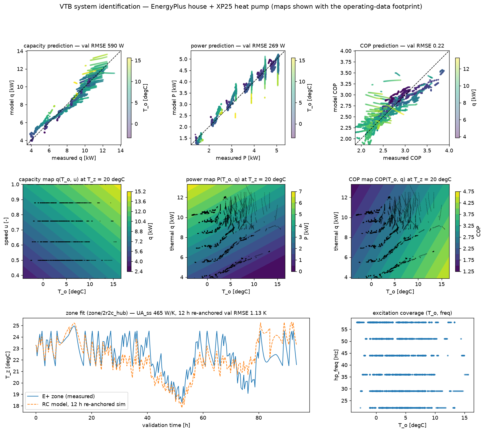
The 2R2C zone model reaches a 1.13 K validation RMSE at the 12-hour re-anchored horizon, versus 1.79 K for 1R1C. The order matters for control, not just fit: 1R1C cannot separate the fast control gain (K per kW over minutes) from slow storage (hours), so a planner built on it materially over-pre-heats (observed as daily 2 K overshoots). The identified second node turned out to be pure internal mass with a direct loss path — a data-driven confirmation of the house’s thermal topology. The equipment maps validate to 590 W (capacity), 269 W (power), and 0.22 (COP) RMSE.
Closed-loop result
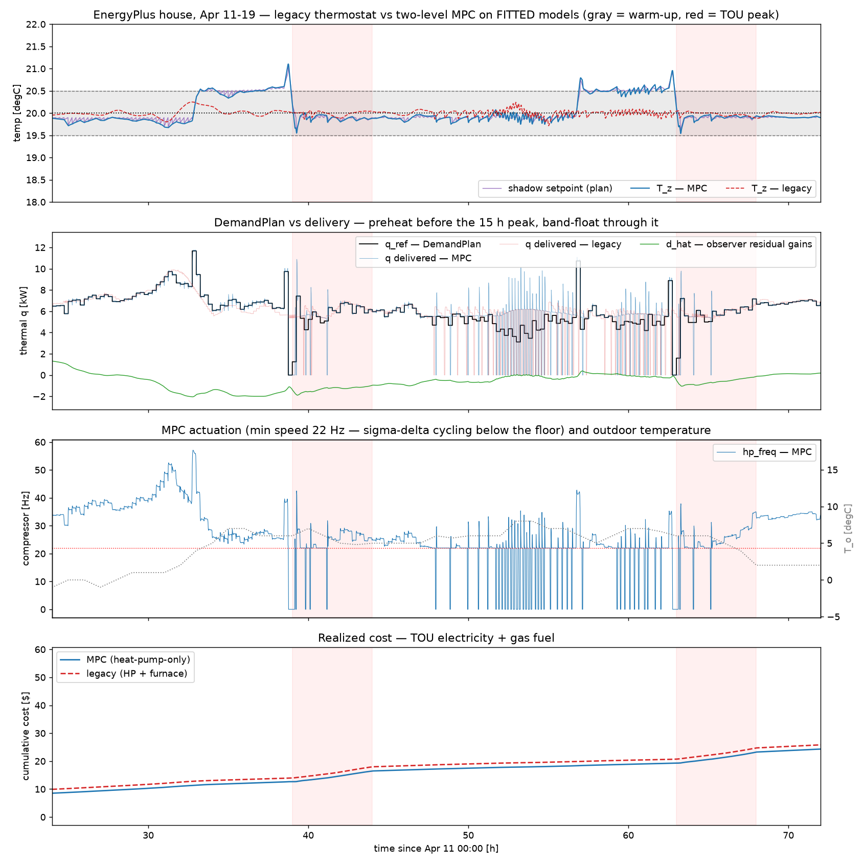
The MPC pre-heats before the 15:00 time-of-use peak, coasts through the peak with the compressor off, and band-floats the rest of the day — while every on/off run honors the 3-minute dwell and the controller stays heat-pump-only (the expensive furnace never fires). Over 7 out-of-sample KPI days (setpoint 20 °C, ±0.5 K band, TOU tariff \$0.45 peak / \$0.10 off-peak per kWh, 15:00–20:00 peak):
| KPI (7 out-of-sample days) | Two-level MPC | Legacy thermostat |
|---|---|---|
| Realized energy cost (TOU elec + gas) | \$47.66 (−0.6 %) | \$47.95 |
| Peak-window energy (15:00–20:00) | 45.5 kWh (−3.1 %) | 46.9 kWh |
| Total electricity | 317.5 kWh | 315.4 kWh |
| Comfort violation (K·h below band) | 0.00 | 0.00 |
| Compressor starts / day | 30.7 (−15 %) | 36.1 |
| Fuel used | heat-pump only | heat-pump only |
Shadow-setpoint tracking in the regulating regime holds a 0.02 K median error (0.20 K at p99), and the safety fallback was never triggered across the entire week. Eight quantitative gates — fit quality, comfort, cost, peak shift, dwell, tracking, and heat-pump-only operation — all pass and gate the demo’s exit code.
The margins here are deliberately honest: April in Utica is mild, so the zone–ambient gradient is small, storage to exploit is limited, and both controllers already run heat-pump-only. What the testbed demonstrates is the mechanism working end-to-end — load shifted out of the priced peak and 15 % less compressor cycling at equal comfort — produced entirely by models learned from data feeding an optimizer, with a fallback that stood ready but never had to intervene. That is the property that generalizes to colder climates, dual-fuel homes, and grid-services (VPP) events, where the arbitrage is far larger.
This is applied R&D on next-generation thermostat autonomy. The architecture and formulation are summarized here at a methodological level; the implementation and product-specific calibration are proprietary.