Overview#

• BFS in Lecture 9 can find the shortest path in graph G from given source s. But it only usable for unit-weighted graph, where the weights of all edges are 1. The distance of each vertex v in terms of s is counted by the number of edges between s and v.

• BFS is a single source shortest-paths problem

Variants#

• in shortest-paths problem, we are given a weighted, directed graph $G=(V,E)$ with weight function w mapping edges to real-valued weights.

  • the weight of a path p=(v0, v1, v2,..., vk) as w(p) is the sum of weights of its constituent edges: $w(p)=\sum _{i=1}^{k}w(v_{i-1},v_i)$

  • define the shortest-path weight $\delta (u,v)$ from $u$ to $v$ by $\delta (u,v)=minw(p):u\to v\text{if path exist else}\mathrm{\infty }$

  • a shortest path from $u$ to $v$ is then defined as any path p with weight $w(p) = \delta(u,v).

• single-destination shortest-paths problem: find a shortest path to a given destination vertex $t$ from each vertex $v$. We can reverse the directoin of each edges in the graph, and reduce this problem to a single-source problem.

• single-pair shortest-path problem: Find a shortest path from $u$ to $v$ for given vertices $u$ and $v$. If we solve the single-source problem with source vertex $u$, we solve this problem also.

• all-pairs shortest-paths problem: Find a shortest path from $u$ to $v$ for every pair of vertices $u$ and $v$. Although we can solve this problem by running a single- source algorithm once from each vertex, we usually can solve it faster. (later in XXX)

Negative-weight edges#

• Negative-weight cycles:

  • the weight of the cyclic path is negative

  • If the graph contains a negative-weight cycle reachable from $s$, however, shortest-path weights are not well defined.

  • No path from $s$ to a vertex on the cycle can be a shortest path—we can always find a path with lower weight by following the proposed “shortest” path and then traversing the negative-weight cycle.

  • If there is a negative-weight cycle on some path from $s$ to $v$, we define $\delta (s,v)=\mathrm{\infty }$.

• Some shortest-paths algorithms, such as Dijkstra’s algorithm, assume that all edge weights in the input graph are nonnegative, as in the road-map example.

• Others, such as the Bellman-Ford algorithm, allow negative-weight edges in the in- put graph and produce a correct answer as long as no negative-weight cycles are reachable from the source.

• Typically, if there is such a negative-weight cycle, the algorithm can detect and report its existence.

Representing shortest paths#

• similar to BFS trees

• shortest paths are not necessarily unique, and neither are shortest-trees.

Relaxation#

• for each vertex $v\in V$, we maintain an attribute $v.d$, which is an upper bound on the weight of a shortest path from source $s$ to $v$.

• initialize the shortest-path estimates and predecessors in $o(V)$ time

   def initialize_single_source(G,s):
       for v in G.V:
           v.d = infinity
           v.p = None
       s.d = 0

• The process of relaxing an edge $(u,v)$ consists of testing whether we can improve the shortest path to $v$ found so far by going through $u$ and, if so, updating $v.d$ and $v.p$.

    def relax(u,v,w):
        if v.d > u.d + w(u,v):
            v.d = u.d + w(u,v)
            v.p = u

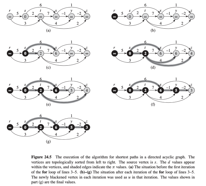
Single-source shortest paths in DAG (directed acyclic graphs)#

• Find the shortest paths from source $s$ to every vertex $v$ in a weighted DAG

• Algorithm: $O(V+E)$ in aggregated analysis

   def DAG_shortest_paths(G, s):
       linked_list = topological_sort(G)
       initialize_single_source(G,s)
       for u in linked_list:
           for v in G.Adj[u]:
               relax(u,v,w)

• Example

• Follow up:

  • How to find the longest path in a DAG?

    • negate the edge weights and runing DAG_shortest_paths(G,s)

    • or modify DAG_shortest_paths(G,s) by replacing $\mathrm{\infty }$ by $-\mathrm{\infty }$ during initialization and $>$ by $<$ in the relax program.